Terrain attributes#
xDEM can derive a wide range of terrain attributes from a DEM.
Attributes are derived in pure Python for modularity (e.g., varying window size) and other uses (e.g., uncertainty), and tested for consistency against gdaldem where relevant.
Quick use#
Terrain attribute methods can be derived either directly from a DEM using slope(), or from an array using the module function xdem.terrain.slope().
# Slope from DEM method
slope = dem.slope()
# Or from terrain module using an array input
slope = xdem.terrain.slope(dem.data, resolution=dem.res)
Tip
All attributes can be derived using either SciPy (default) or Numba (optional dependency) as computing engine.
Both perform similarly, with Numba usually being slightly faster (x2 to 4) for deriving multiple times the same attributes, due to optimization for your machine at the cost of an initial compile time (usually lasting about 5 to 10 seconds). See Numba’s just-in-time compilation and compilation caching for details.
For optimal speed of windowed attributes on SciPy, ensure that you are using SciPy 1.16 or later (with vectorized_filter available).
Summary of supported methods#
xDEM currently supports three types of terrain attributes: surface fit attributes that rely on estimating local derivatives (e.g. slope, aspect, curvatures), windowed attributes that rely on estimating local indexes often applicable to any window size (e.g., TPI, roughness), and frequency attributes that rely on estimating relative frequency over the whole DEM (e.g. texture shading).
Note that curvatures follow the recommended system of Minár et al. (2020). Where no direct DOI can be linked, consult this paper for the full citation.
Attribute |
Unit (if DEM in meters) |
Reference |
|---|---|---|
Degrees (default) or radians |
||
Degrees (default) or radians |
||
Unitless |
||
Meters-1 * 100 |
Krcho (1973) and Evans (1979) (geometric) or Zevenbergen and Thorne (1987) (directional) |
|
Meters-1 * 100 |
Krcho (1983) (geometric) or Zevenbergen and Thorne (1987) (directional) |
|
Meters-1 * 100 |
Sobolevsky (1932) (geometric and directional) |
|
Meters-1 * 100 |
Minár et al. (2020) (geometric) or Shary (1991) (directional) |
|
Meters-1 * 100 |
Shary (1995) (geometric) or Wood (1996) (directional) |
|
Meters-1 * 100 |
Shary (1995) (geometric) or Wood (1996) (directional) |
|
Meters |
||
Meters |
||
Meters |
||
Unitless |
||
Fractal dimension number (1 to 3) |
||
Unitless |
Note
Only grids with equal pixel size in X and Y are currently supported. Transform into such a grid with reproject().
Surface fit attributes#
Primer on partial derivatives of elevation#
Most of the terrain attributes below are calculated from partial derivatives of elevation. Our terminology follows that of Minár et al. (2020), whereby the surface elevation \(z\) can be expressed as the function
where \(x\) and \(y\) are Cartesian coordinates. First- and second-order partial derivatives of elevation are defined as follows:
xDEM offers multiple methods of calculating these partial derivatives, which can be set using the surface_fit parameter:
"Horn": Derivatives are calculated based on a refined gradient formulation of a 3 \(\times\) 3 pixel window following Horn (1981),"ZevenbergThorne": Derivatives are calculated based on a partial quartic polynomial fit to a 3 \(\times\) 3 pixel window following Zevenbergen and Thorne (1987),"Florinsky": Derivatives are calculated based on a third-order polynomial fit to a 5 \(\times\) 5 pixel window following Florinsky (2009).
By default, "Florinsky" is used, as this provides opportunities for higher-order derivatives and the 5 \(\times\) 5 pixel fit is theoretically more robust to noise than a 3 \(\times\) 3 pixel fit. Note that "Horn" only calculates \(z_{x}\) and \(z_{y}\) derivatives, and as such cannot be used for advanced terrain attributes such as curvatures.
The differences between methods are illustrated in the Slope and aspect methods example.
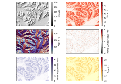
Slope#
The slope of a DEM describes the tilt, or gradient, of each pixel in relation to its neighbours. It is most often described in degrees, where a flat surface is 0° and a vertical cliff is 90°. No tilt direction is stored in the slope map; a 45° tilt westward is identical to a 45° tilt eastward.
The slope \(\alpha\) is defined as
and the surface derivatives can be computed either by the method of Horn (1981), Zevenbergen and Thorne (1987), or Florinsky (2009) (default).
slope = dem.slope(surface_fit="Florinsky")  # "Florinsky" is default
slope.plot(cmap="Reds", cbar_title="Slope (°)")
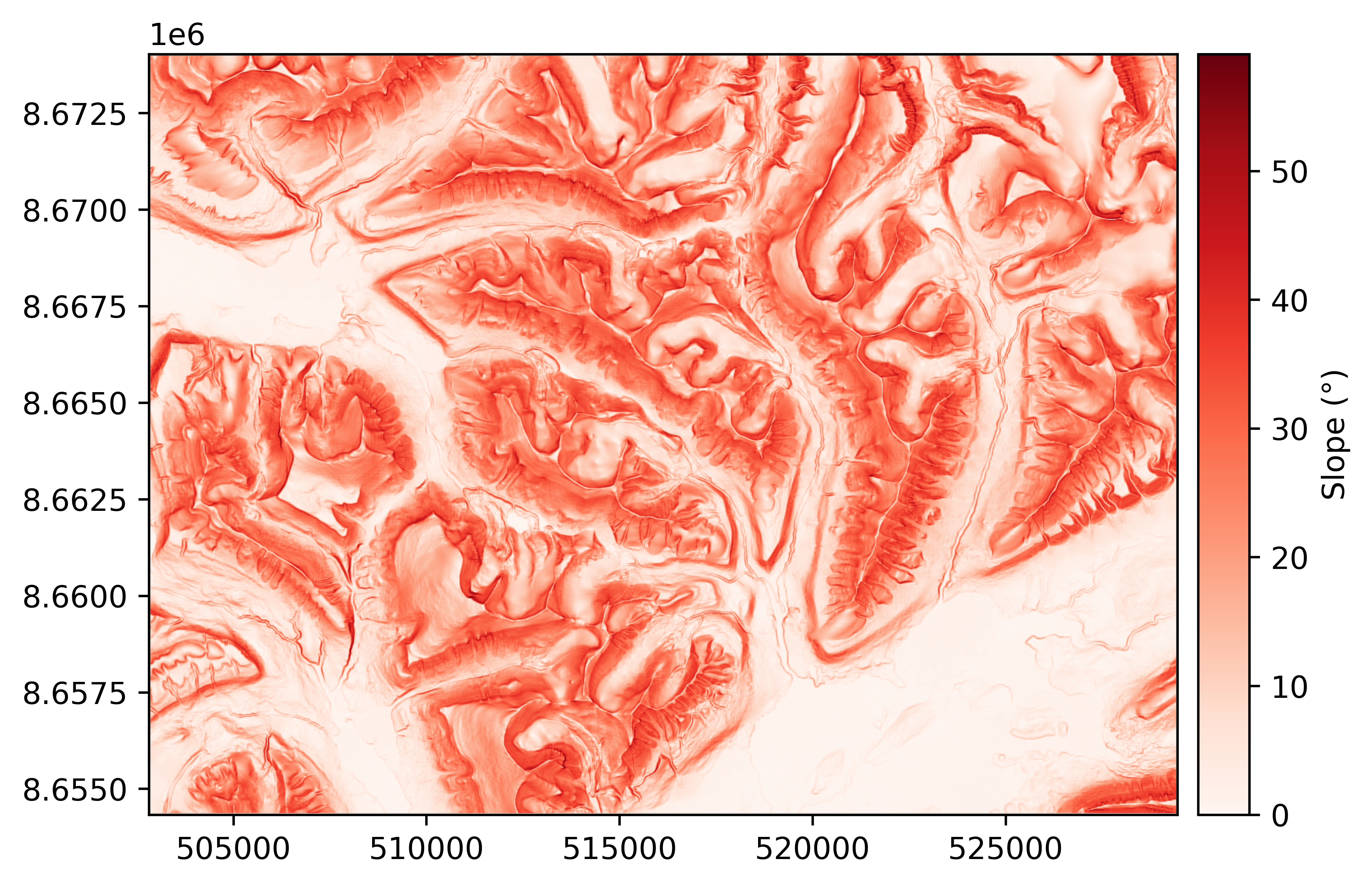
Aspect#
The aspect describes the orientation of strongest slope. It is often reported in degrees, where a slope tilting straight north corresponds to an aspect of 0°, and an eastern aspect is 90°, south is 180° and west is 270°. By default, a flat slope is given an arbitrary aspect of 180°.
The aspect \(\theta\) is defined as
Like with slope, the surface derivatives can be calculated following the methods of Horn (1981), Zevenbergen and Thorne (1987), or Florinsky (2009) (default).
Warning
A north aspect represents the upper direction of the Y axis in the coordinate reference system of the
input, xdem.DEM.crs, which might not represent the true north.
aspect = dem.aspect()
aspect.plot(cmap="twilight", cbar_title="Aspect (°)")
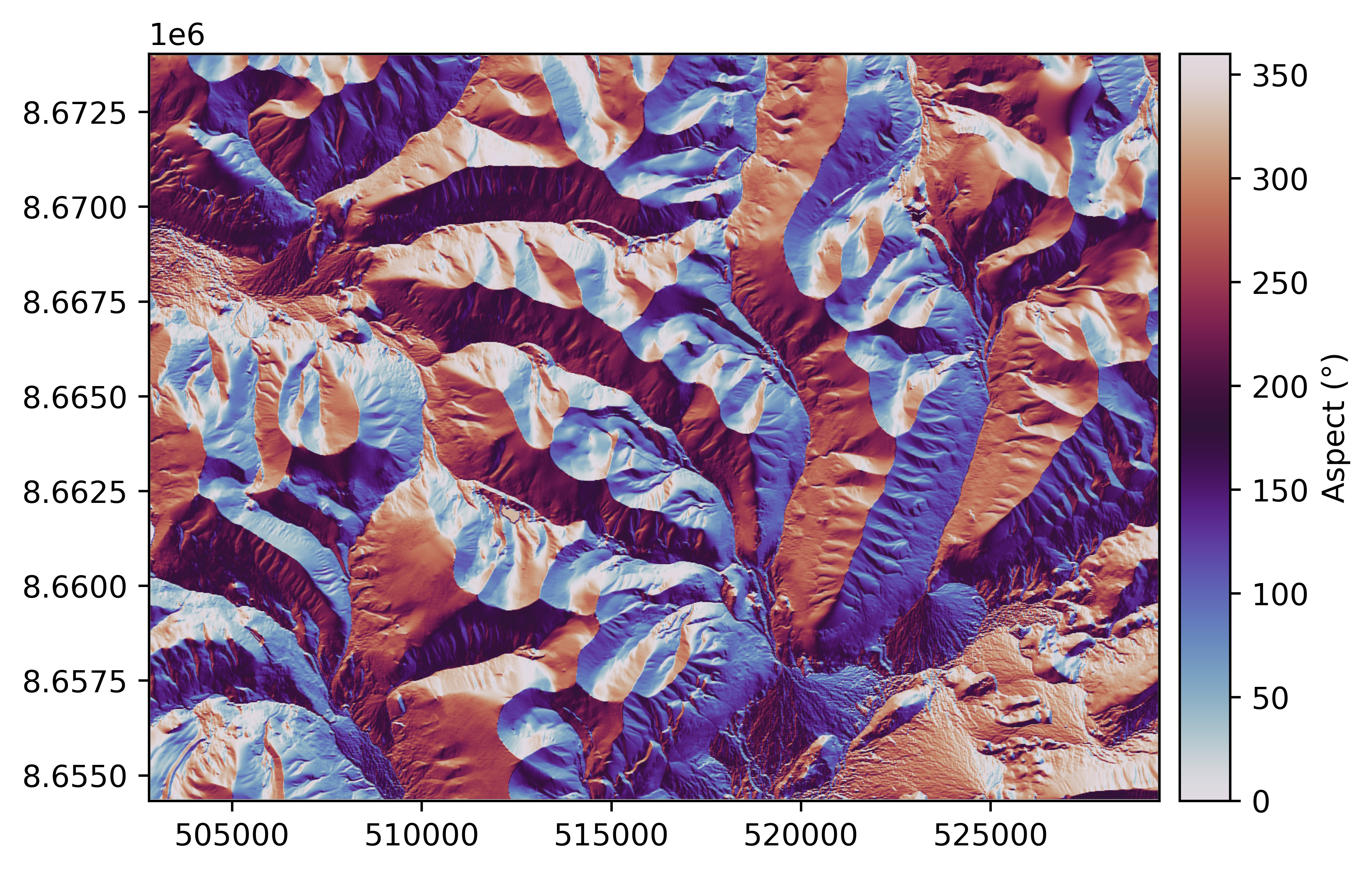
Hillshade#
The hillshade is a slope map, shaded by the aspect of the slope. With a westerly azimuth (a simulated sun coming from the west), all eastern slopes are slightly darker. This mode of shading the slopes often generates a map that is much more easily interpreted than the slope.
The hillshade \(hs\) is directly based on the slope \(\alpha\) and aspect \(\theta\), and thus also varies between the methods of Horn (1981), Zevenbergen and Thorne (1987), and Florinsky (2009) (default). It is often scaled between 1 and 255:
where \(alt\) is the shading altitude (90° = from above) and \(azim\) is the shading azimuth (0° = north).
Note, however, that the hillshade is not a shadow map; no occlusion is taken into account so it does not represent “true” shading. It therefore has little analytic purpose, but it still constitutes a great visualization tool.
hillshade = dem.hillshade()
hillshade.plot(cmap="Greys_r", cbar_title="Hillshade")
Curvatures#
Curvatures are the second derivative of elevation, aiming to describe the convexity or concavity of a terrain. If a surface is convex (like a mountain peak), it will have positive curvature. If a surface is concave (like a through or a valley bottom), it will have negative curvature.
There are countless possible curvatures to calculate, the most common of which we provide functions for. Terminology in the literature are confusing, with the same terms (e.g. “horizontal curvature”) often referring to different mathematical definitions. For consistency, we follow the terminology of Minár et al. (2020). We provide the six basic curvatures (profile, tangential, planform, flowline, maximal/maximum, and minimal/minimum). These form the basis from which several others (e.g. mean, unsphericity) may be calculated easily (sum, difference).
There are two parallel systems of defining curvatures: either geometric (curvatures can be defined by the radius of a circle), or directional derivative (curvatures can be understood as directional derivatives of the elevation field). For more information on this, Minár et al. (2020) provides a comprehensive review. The choice of system can be set in xDEM via the curv_method parameter. This defaults to the "geometric" method, which should be suitable for most users, although "directional" is also available for those interested.
All curvatures require \(z_{xx}\), \(z_{xy}\), and/or \(z_{yy}\) partial derivatives: as a result, only Zevenbergen and Thorne (1987), and Florinsky (2009) surface fit methods can be used. By default, "Florinsky" is used.
The curvature values in units of m-1 are quite small, so they are by convention multiplied by 100.
We are grateful to Ian Evans and Josef Minár for their guidance and recommendations in providing a consistent and sensible set of curvature options.
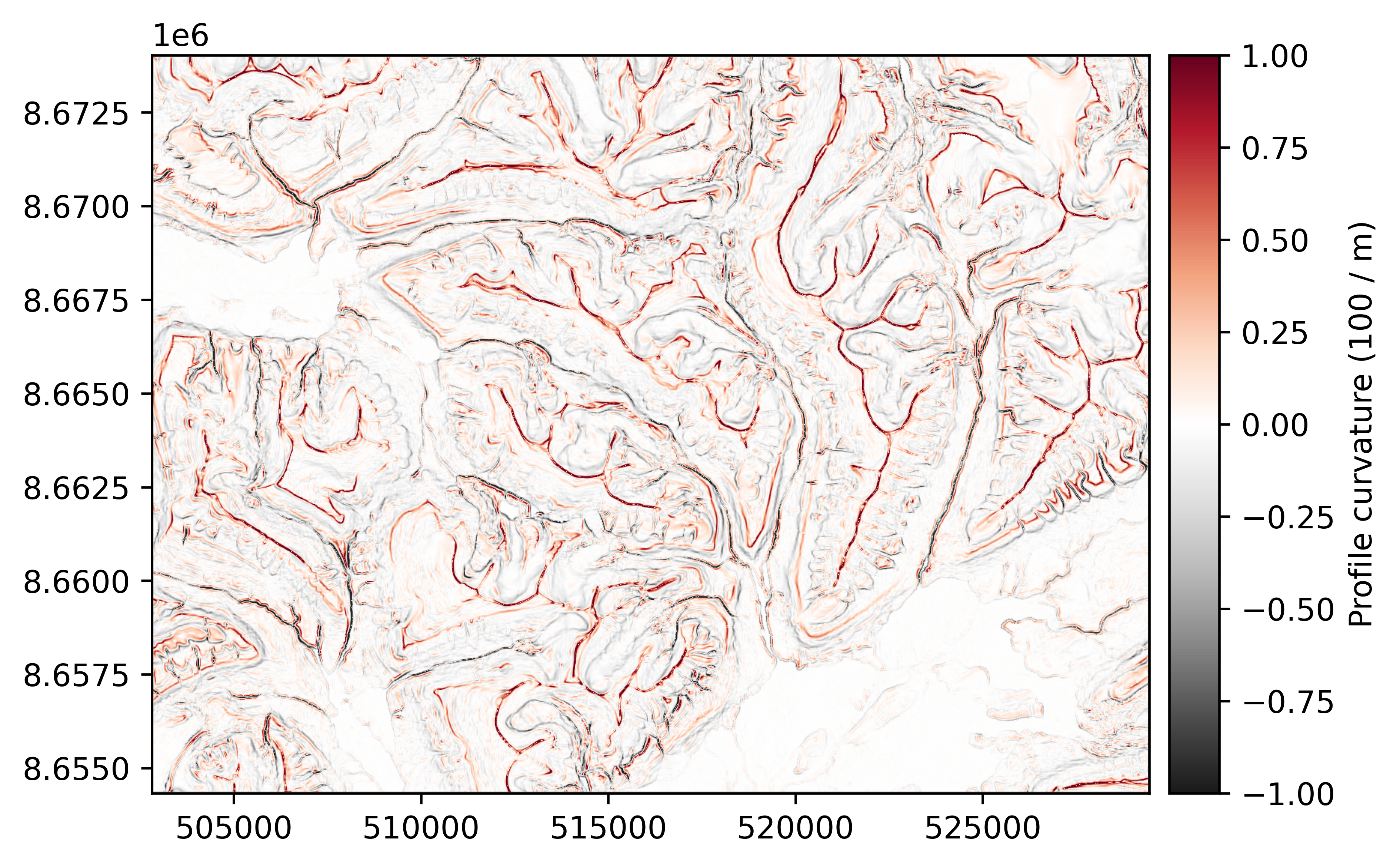
Profile curvature#
The profile curvature is the curvature of a normal section of slope that is tangential to the slope line (i.e. the curvature along the direction of steepest slope at a point).
The geometric (default) method follows Krcho (1973) and Evans (1979) as outlined in Minár et al. (2020):
while the directional derivative method follows Zevenbergen and Thorne (1987):
profile_curvature = dem.profile_curvature()
profile_curvature.plot(cmap="RdGy_r", cbar_title="Profile curvature (100 / m)", vmin=-1, vmax=1, interpolation="antialiased")
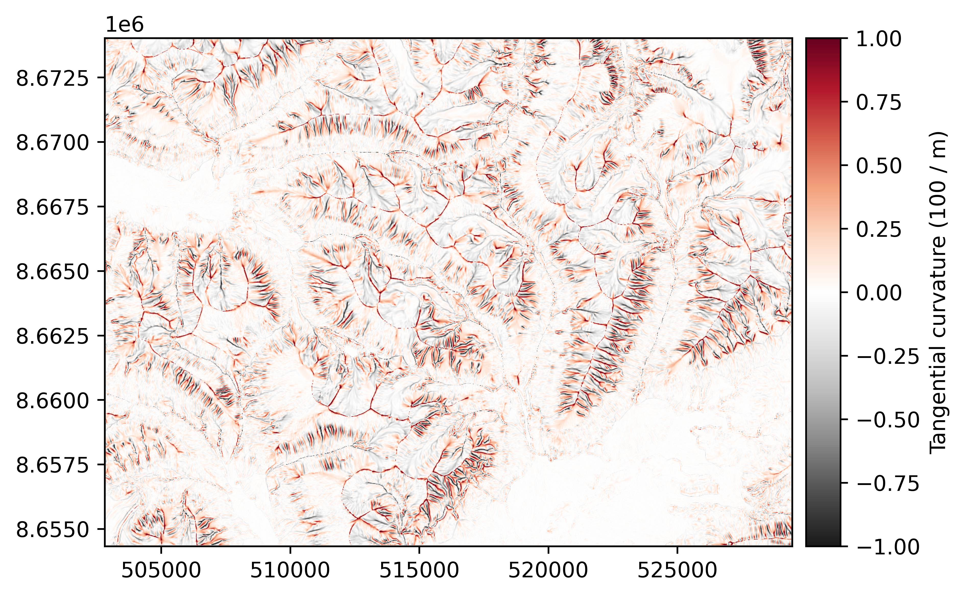
Tangential curvature#
xdem.DEM.tangential_curvature()
The tangential curvature is defined as the curvature of a normal section of slope that is tangential to the contour line. It is sometimes known as the principal, normal contour, or horizontal curvature, although the latter terminology has been shared with planform curvature.
The geometric (default) method follows Krcho (1983) as described in Minár et al. (2020):
while the directional derivative method follows the ‘plan curvature’ of Zevenbergen and Thorne (1987) (although in the Minár terminology, this should not be called the plan or planform curvature):
tangential_curvature = dem.tangential_curvature()
tangential_curvature.plot(cmap="RdGy_r", cbar_title="Tangential curvature (100 / m)", vmin=-1, vmax=1, interpolation="antialiased")
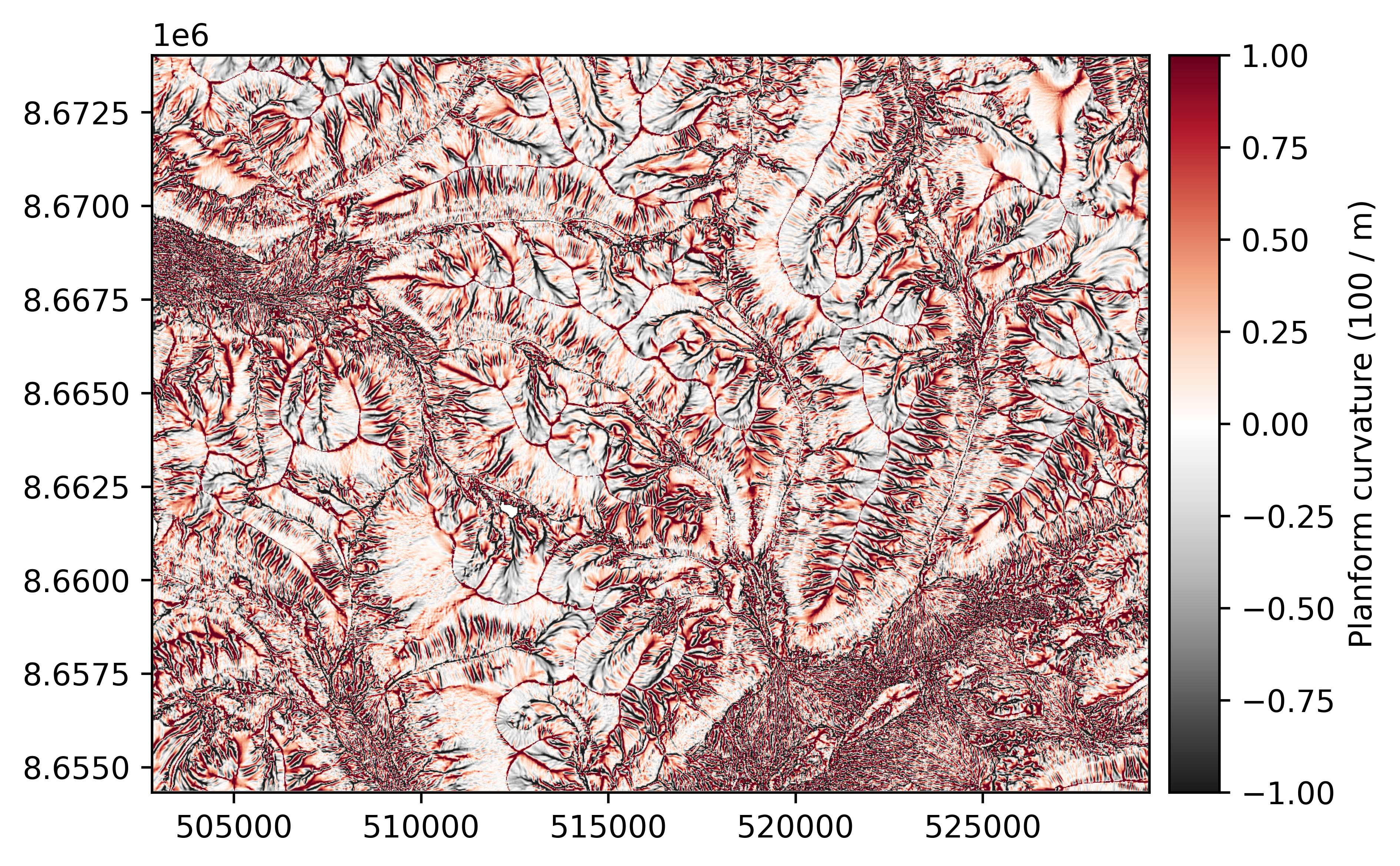
Planform curvature#
The planform (or plan) curvature is defined as the curvature of a projection of the contour line onto a horizontal plane. Sometimes known as the horizontal curvature, although this terminology has been shared with tangential curvature.
This curvature is the same in both the geometric and directional derivative system, and follows Sobolevsky (1932) in Minár et al. (2020):
planform_curvature = dem.planform_curvature()
planform_curvature.plot(cmap="RdGy_r", cbar_title="Planform curvature (100 / m)", vmin=-1, vmax=1, interpolation="antialiased")
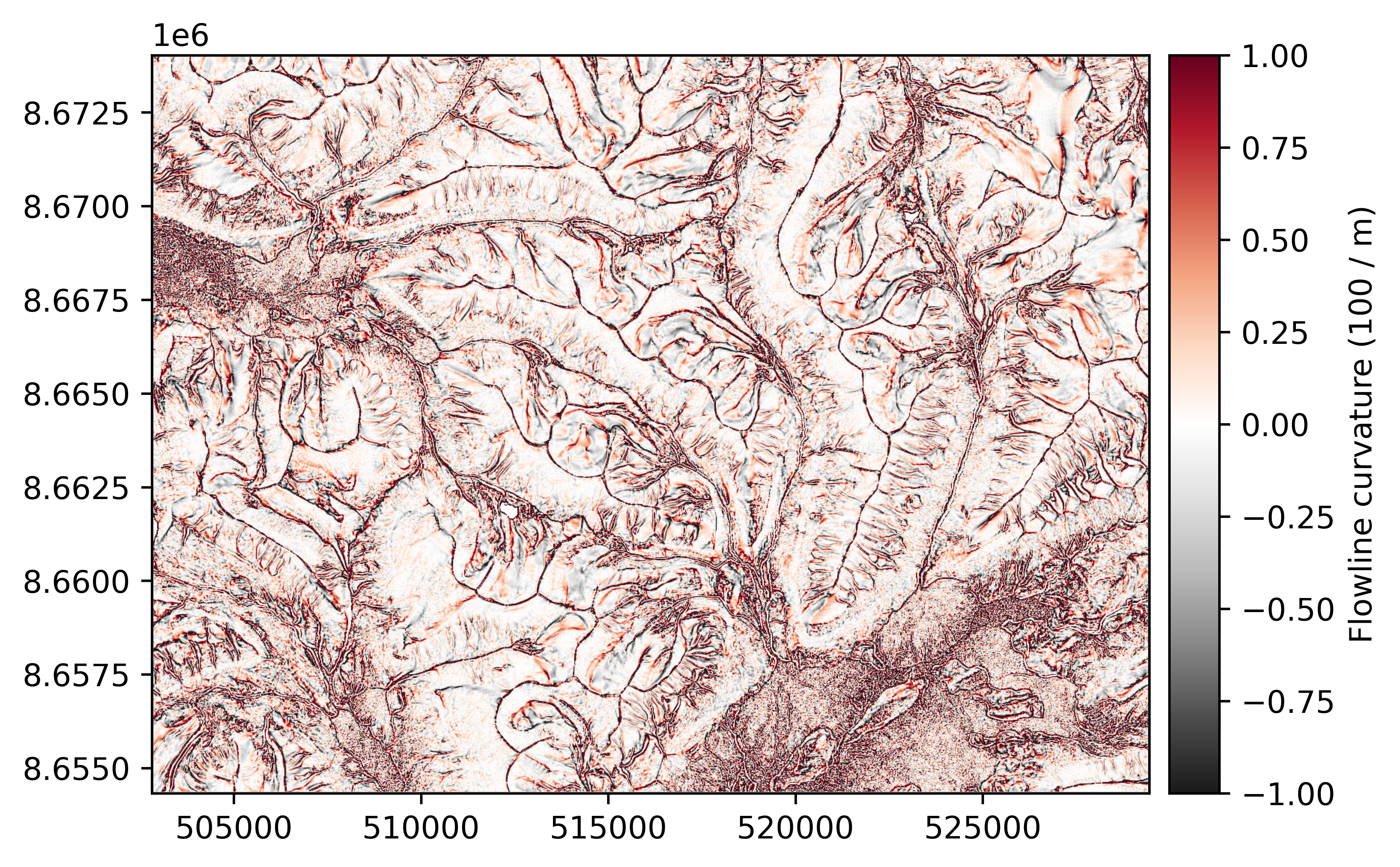
Flowline curvature#
Flowline curvature is defined as the curvature of a projection of the slope line onto a horizontal plane. It is sometimes known as the rotor or stream line curvature.
The geometric (default) flowline curvature follows the “contour torsion” described by Minár et al. (2020):
while the directional derivative flowline curvature follows that of Shary (1991) in Minár et al. (2020):
flowline_curvature = dem.flowline_curvature()
flowline_curvature.plot(cmap="RdGy_r", cbar_title="Flowline curvature (100 / m)", vmin=-1, vmax=1, interpolation="antialiased")
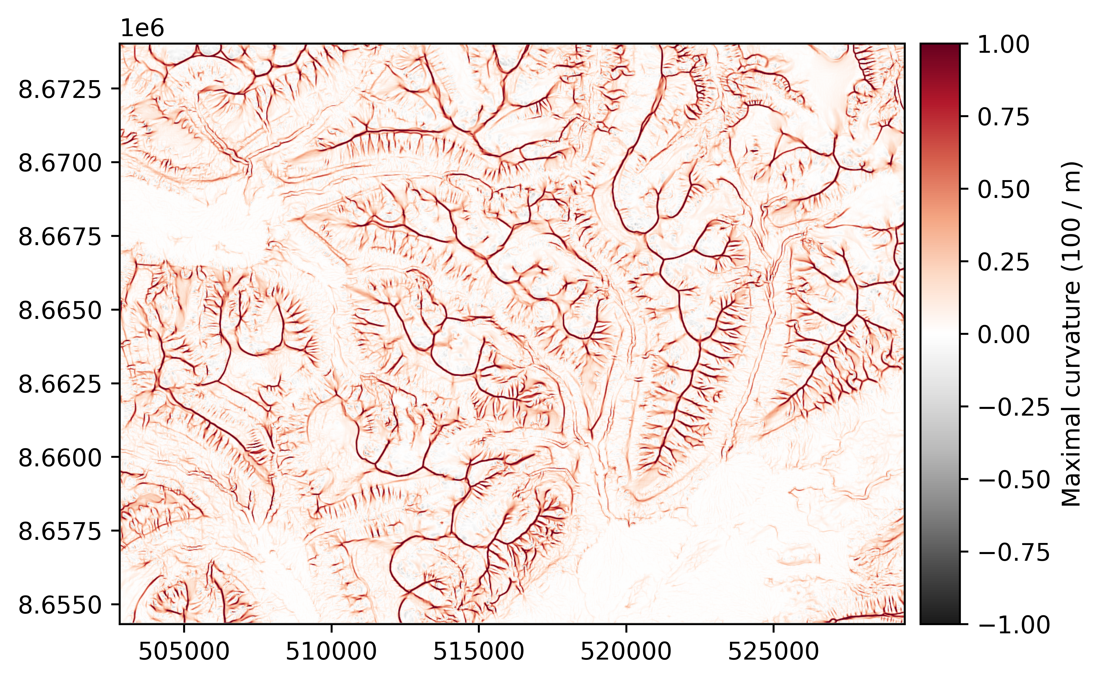
Maximal/maximum curvature#
The maximal (geometric) or maximum (directional derivative) curvature is defined as curvature of the normal section of slope with the greatest curvature value.
The geometric (default) maximal curvature is calculated following Shary (1995), which is equal to the minimal curvature of Euler (1767) (!), and is defined in terms of the mean curvature \(k_{mean}\) and the unsphericity \(k_u\):
while the directional derivative maximum curvature is the minimum second derivative following Wood (1996):
max_curvature = dem.max_curvature()
max_curvature.plot(cmap="RdGy_r", cbar_title="Maximal curvature (100 / m)", vmin=-1, vmax=1, interpolation="antialiased")
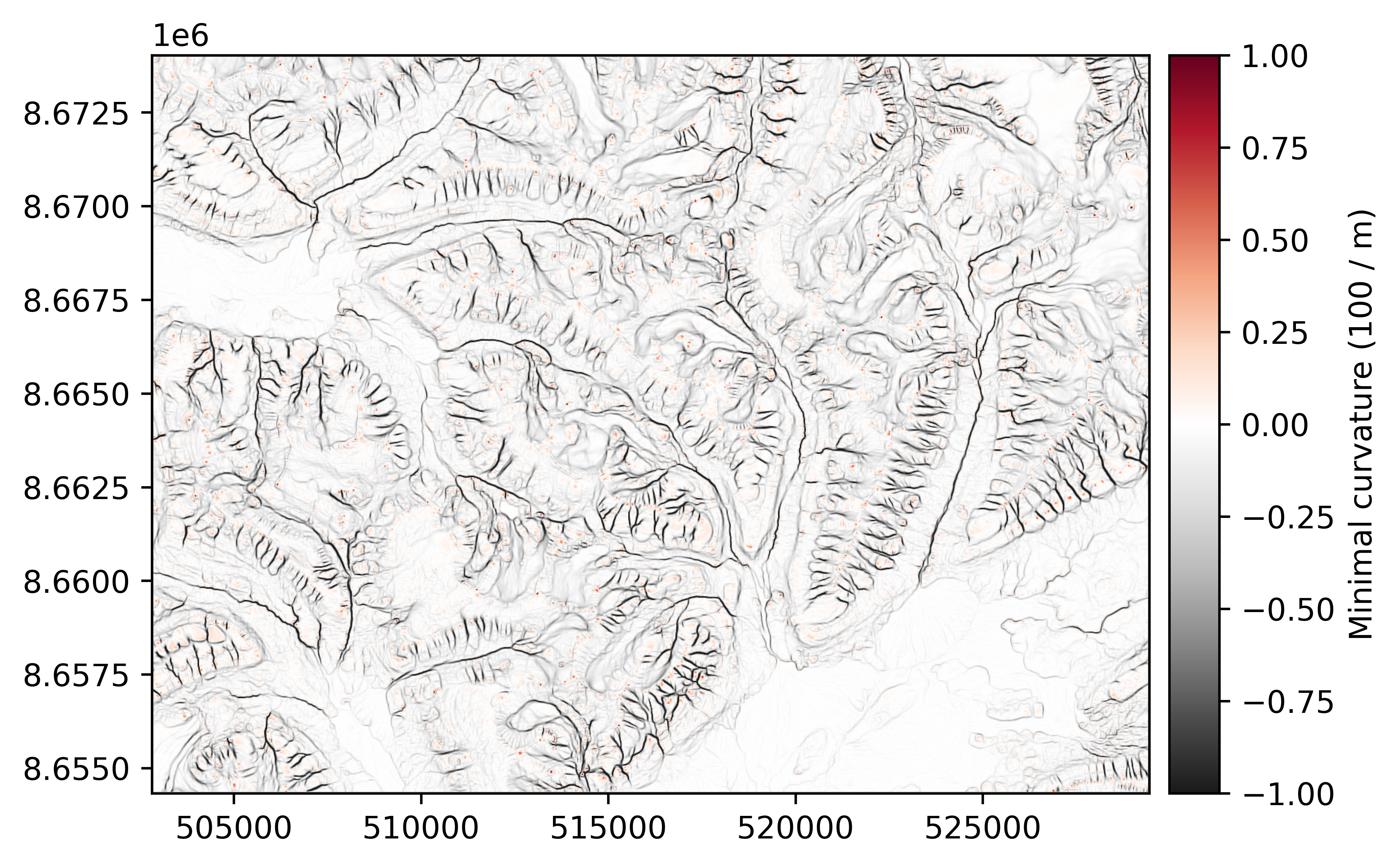
Minimal/minimum curvature#
The minimal (geometric) or minimum (directional derivative) curvature is defined as curvature of the normal section of slope with the lowest curvature value.
The geometric (default) minimal curvature is calculated following Shary (1995), which is equal to the maximal curvature of Euler (1767) (!), and is defined in terms of the mean curvature \(k_{mean}\) and the unsphericity \(k_u\):
while the directional derivative minimum curvature is the maximum second derivative following Wood (1996):
min_curvature = dem.min_curvature()
min_curvature.plot(cmap="RdGy_r", cbar_title="Minimal curvature (100 / m)", vmin=-1, vmax=1, interpolation="antialiased")
Windowed attributes#
xDEM supports a wide range of windowed attributes, for which the calculations are based solely on the distribution of pixels within a window.
In the following, we describe these attributes using the annotation \(z_{ij}\) for pixels, centered on \(z_{00}\), with a pixel resolution west-east of \(\Delta x\) and south-north of \(\Delta y\). For example, for a 3x3 window could be annotated:
West |
Center |
East |
|
|---|---|---|---|
North |
\(z_{-+}\) |
\(z_{0+}\) |
\(z_{++}\) |
Center |
\(z_{-0}\) |
\(z_{00}\) |
\(z_{+0}\) |
South |
\(z_{--}\) |
\(z_{0-}\) |
\(z_{+-}\) |
The default window size in 3x3 pixels for all attributes, except for fractal roughness that defaults to 11x11 pixels.
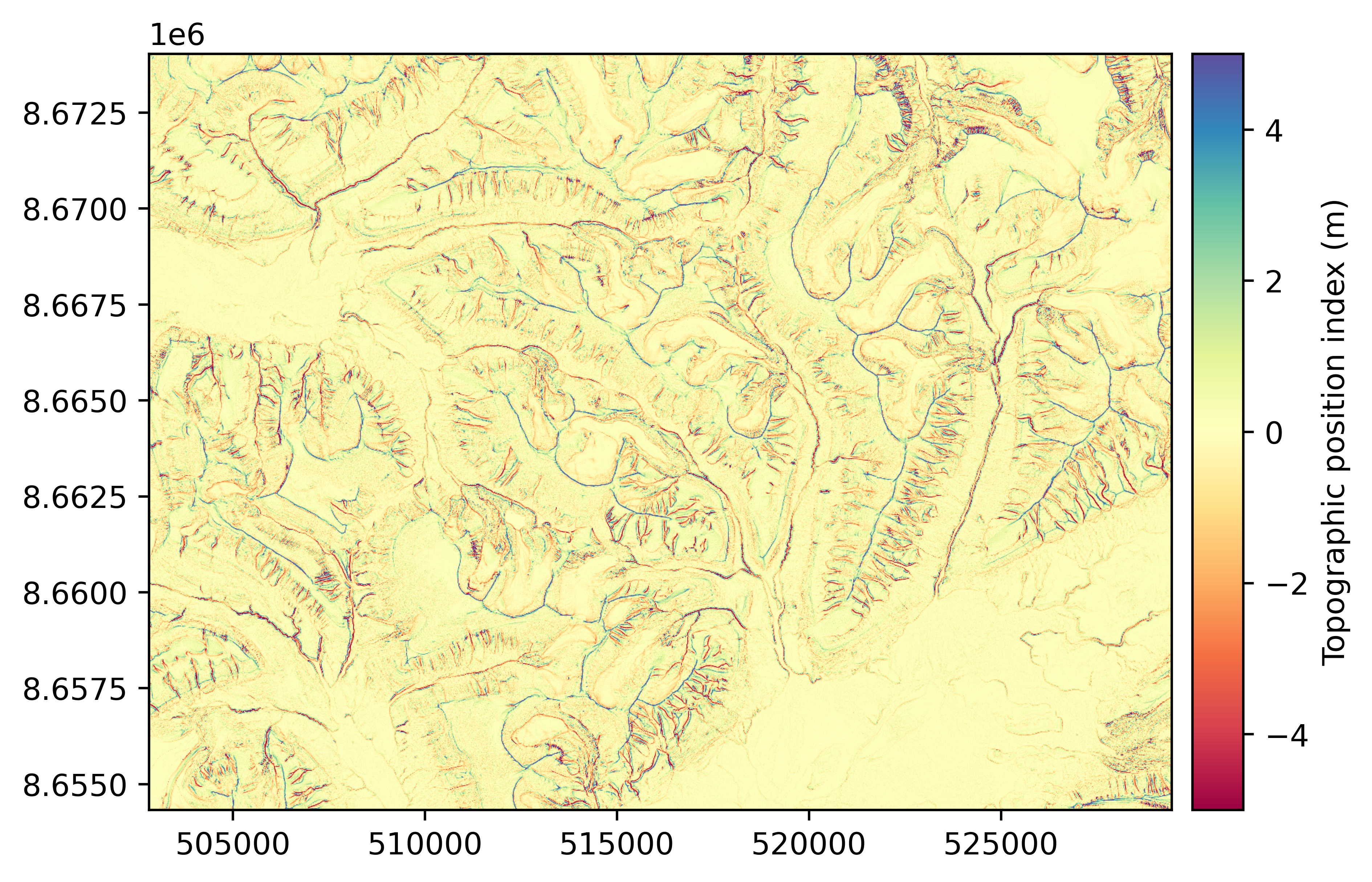
Topographic position index#
xdem.DEM.topographic_position_index()
The topographic position index (TPI) is a metric of slope position, described in Weiss (2001), that corresponds to the difference of the elevation of a central pixel with the average of that of neighbouring pixels. Its unit is that of the DEM (typically meters) and it can be computed for any window size (default 3x3 pixels).
tpi = dem.topographic_position_index()
tpi.plot(cmap="Spectral", cbar_title="Topographic position index (m)", vmin=-5, vmax=5)
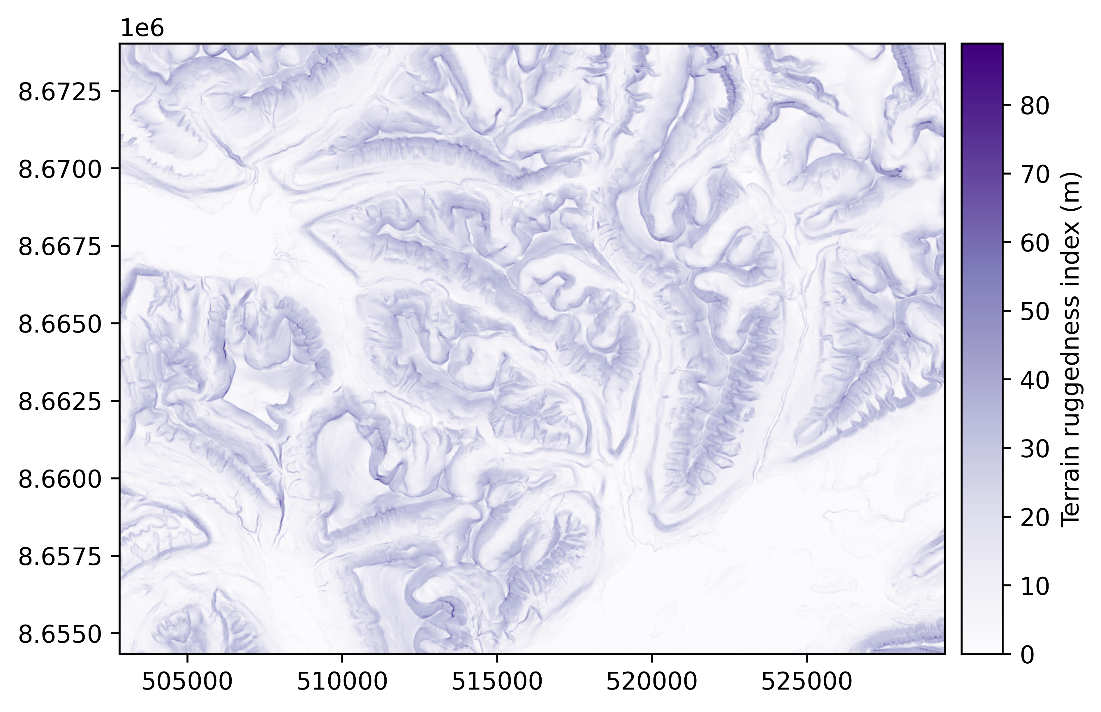
Terrain ruggedness index#
xdem.DEM.terrain_ruggedness_index()
The terrain ruggedness index (TRI) is a metric of terrain ruggedness, based on cumulated differences in elevation between a central pixel and its surroundings. Its unit is that of the DEM (typically meters) and it can be computed for any window size (default 3x3 pixels).
For topography (default), the method of Riley et al. (1999) is generally used, where the TRI is computed by the squareroot of squared differences with neighbouring pixels:
For bathymetry, the method of Wilson et al. (2007) is generally used, where the TRI is defined by the mean absolute difference with neighbouring pixels:
tri = dem.terrain_ruggedness_index()
tri.plot(cmap="Purples", cbar_title="Terrain ruggedness index (m)")
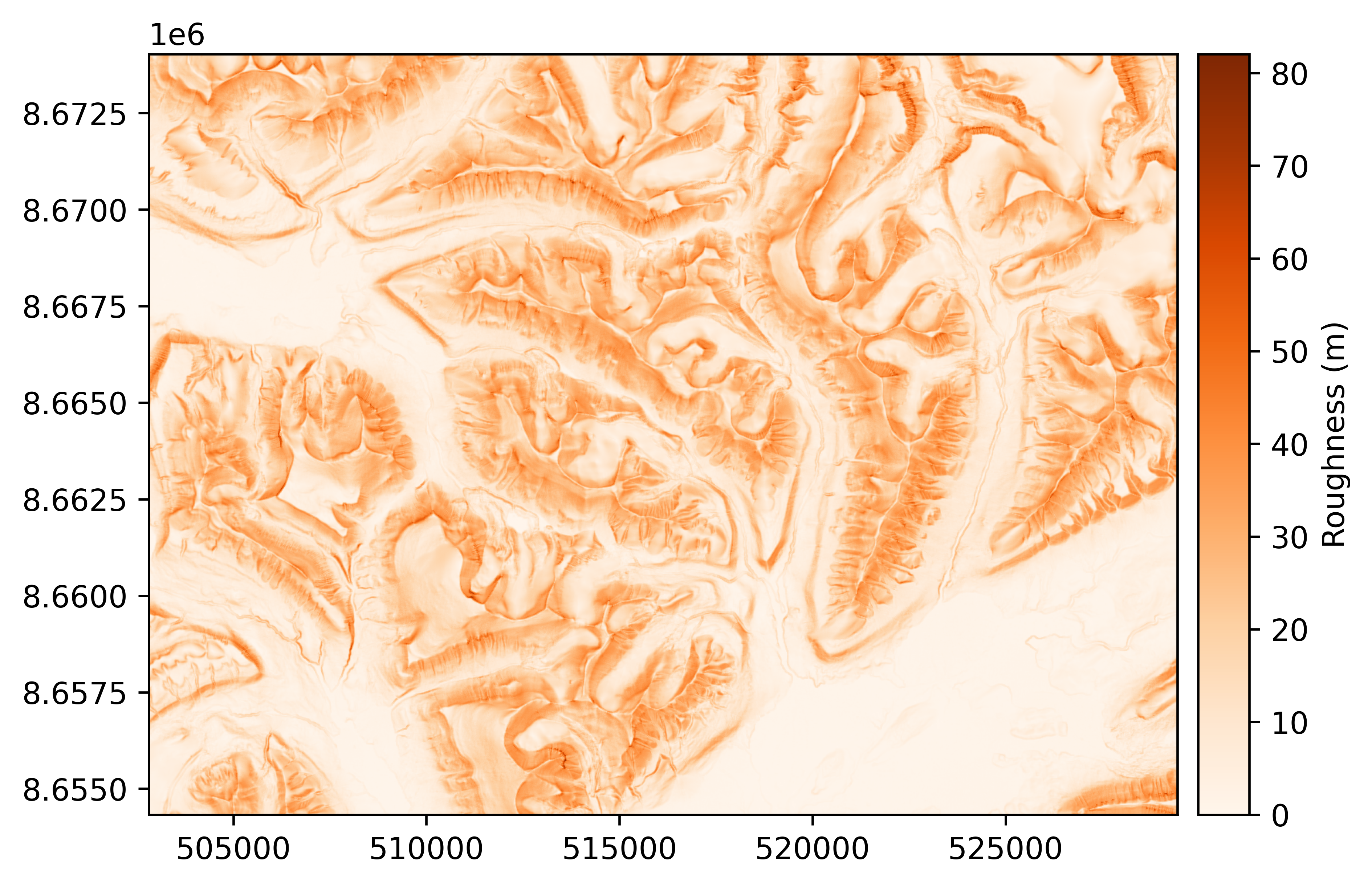
Roughness#
The roughness is a metric of terrain ruggedness, based on the maximum difference in elevation in the surroundings, described in Dartnell (2000). Its unit is that of the DEM (typically meters) and it can be computed for any window size (default 3x3 pixels).
roughness = dem.roughness()
roughness.plot(cmap="Oranges", cbar_title="Roughness (m)")
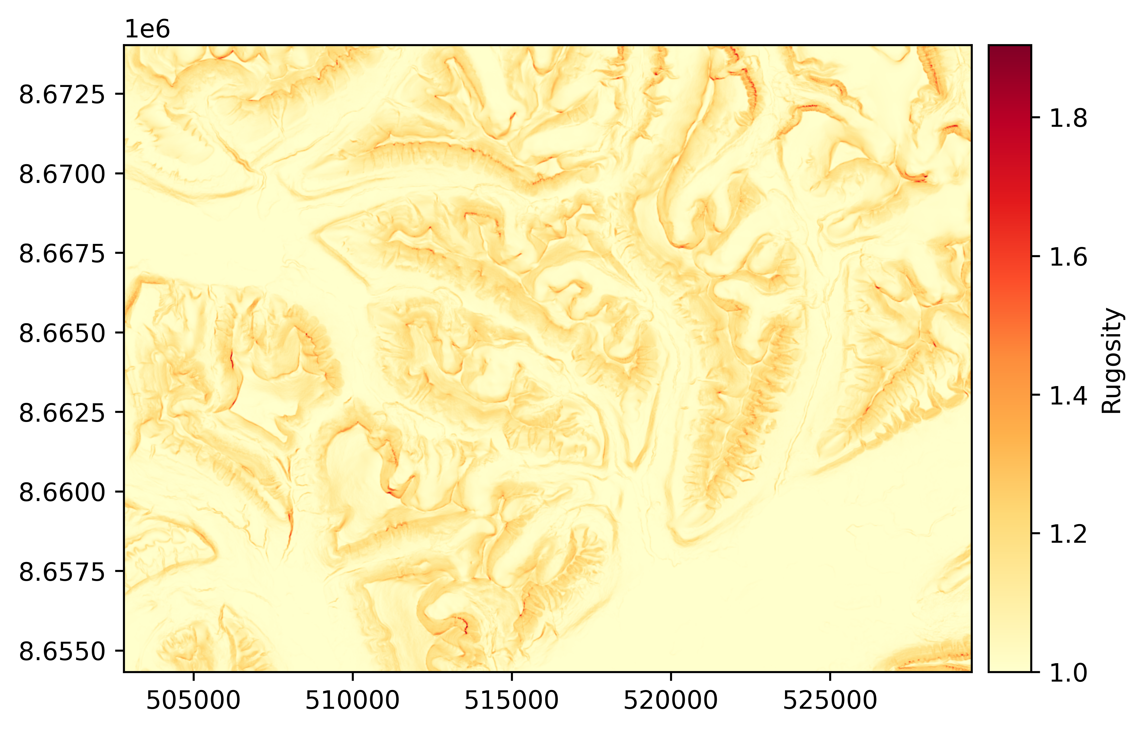
Rugosity#
The rugosity is a metric of terrain ruggedness, based on the ratio between planimetric and real surface area, described in Jenness (2004). It is unitless, and is only supported for a 3x3 window size.
where \(A(T_{00,k})\) is the area of one of the 8 triangles connected from the center of the center pixel \(00\) to the centers of its 8 neighbouring pixels \(k\), cropped to intersect only the center pixel. This surface area is computed in three dimensions, accounting for elevation differences.
rugosity = dem.rugosity()
rugosity.plot(cmap="YlOrRd", cbar_title="Rugosity")
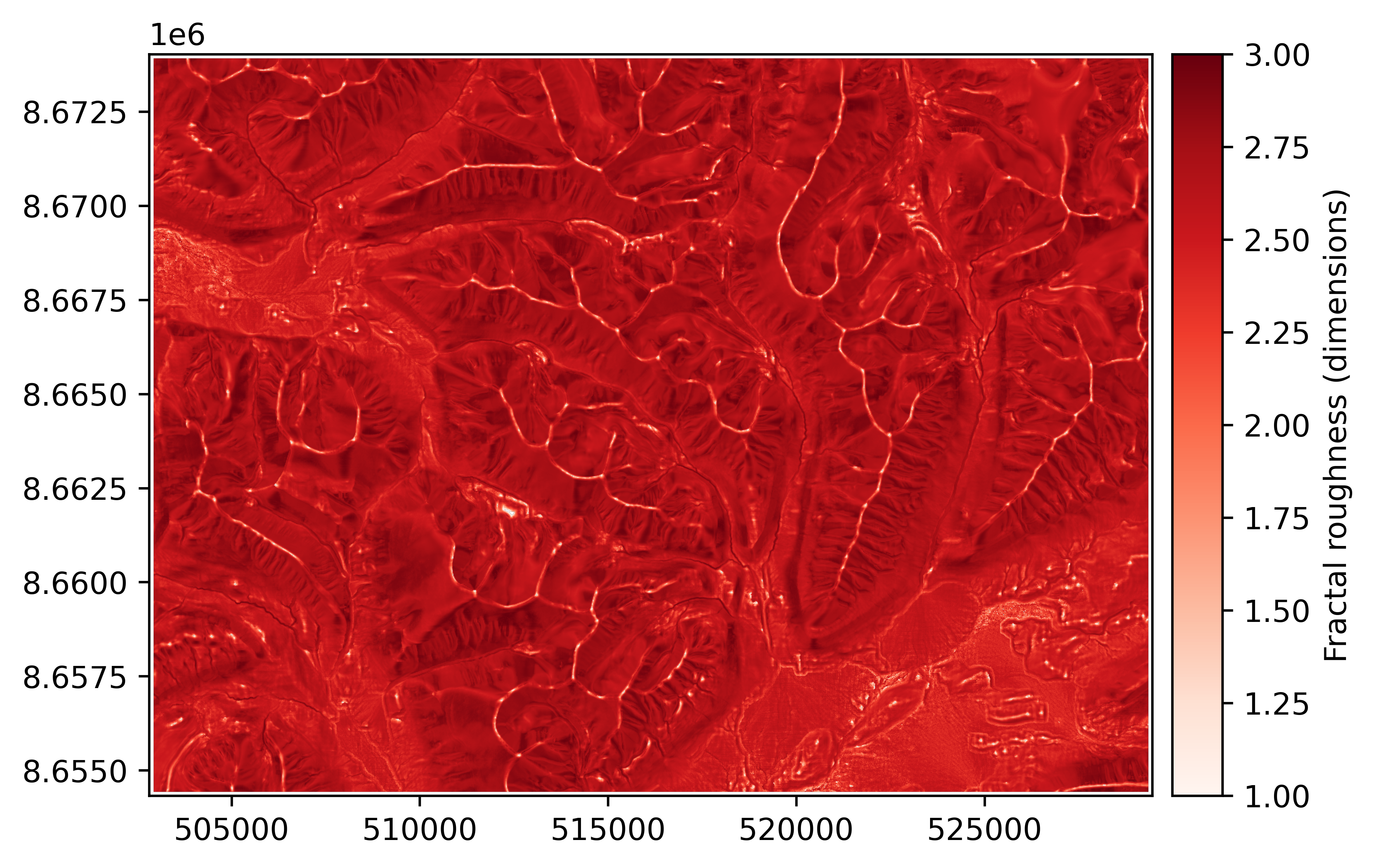
Fractal roughness#
The fractal roughness is a metric of terrain ruggedness based on the local fractal dimension estimated by the volume box-counting method of Taud and Parrot (2005). The fractal roughness is computed by estimating the fractal dimension in 3D space, for a local window centered on the DEM pixels. Its unit is that of a dimension, and is always between 1 (dimension of a line in 3D space) and 3 (dimension of a cube in 3D space). It can only be computed on window sizes larger than 5x5 pixels, and defaults to 13x13.
fractal_roughness = dem.fractal_roughness()
fractal_roughness.plot(cmap="Reds", cbar_title="Fractal roughness (dimensions)")
Frequency attributes#
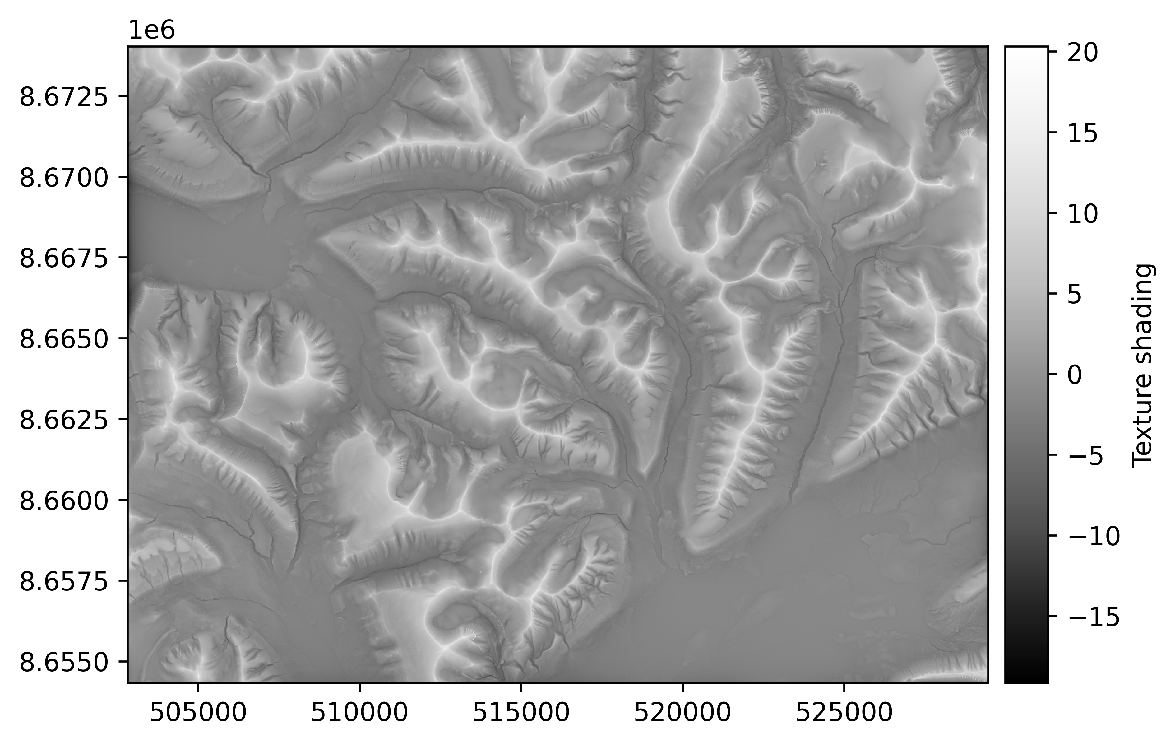
Texture shading#
The texture shading technique produces an isotropic relief visualization that emphasizes the drainage network structure of terrain, including ridges and canyons. Unlike traditional hillshading, texture shading exhibits scale invariance and orientation independence, making it particularly effective for revealing the hierarchical structure of mountainous topography without directional bias.
Texture shading is computed by applying a fractional Laplacian operator to the elevation data, which acts as a scale-independent high-pass filter. The technique produces relative elevation values where positive values correspond to ridges and peaks (higher than surrounding terrain) and negative values correspond to valleys and canyons (lower than surrounding terrain). The method includes a detail parameter α (typically 0.5–1.0) that controls the emphasis given to fine terrain features versus major landscape structure.
The fractional Laplacian operator \(L^{\alpha}\) is based on Brown (2010) and computed in the frequency domain as:
\(L^{\alpha}(f_x, f_y) = (2\pi)^{\alpha} \left( f_x^2 + f_y^2 \right)^\frac{\alpha}{2}\)
where \(f_x\) and \(f_y\) are spatial frequencies, and \(\alpha\) is the fractional order parameter.
Unlike hillshading, texture shading maintains visual hierarchy across different scales—smaller terrain features automatically have lower contrast relative to larger features, creating a “self-generalizing” effect. This makes texture shading particularly valuable for displaying terrain at multiple zoom levels or for combining with traditional hillshading to enhance the visibility of drainage networks.
Unlike curvature, which highlights local convexity and concavity based on the second derivative of elevation, texture shading emphasizes the multi-scale drainage network structure through a fractional Laplacian that preserves relationships across different spatial frequencies. While curvature is optimal for identifying specific geomorphological features like ridges and valley bottoms at a single scale, texture shading provides a scale-invariant visualization that simultaneously reveals both fine-scale terrain details and broad landscape patterns.
For more information on texture shading, see the official texture shading website, the Python implementation reference, and the publication by Allmendinger and Karabinos (2023).
texture_shading = dem.texture_shading(alpha=0.8)
texture_shading.plot(cmap="Greys_r", cbar_title="Texture shading")
Generating attributes in multiprocessing#
Computing terrain attributes over large digital elevation models can be computationally expensive,
especially for high-resolution datasets. To improve performance and reduce memory usage,
xDEM supports multiprocessing for out-of-memory attribute calculations using the mp_config parameter.
The resulting attribute is saved directly to disk under the filename specified in mp_config.
Example#
from geoutils.raster import MultiprocConfig

mp_config = MultiprocConfig(chunk_size=200, outfile="hillshade.tif")
hillshade = dem.hillshade(mp_config=mp_config)
hillshade
Raster(
  data=not_loaded; shape on disk (1, 985, 1332); will load (985, 1332)
  transform=| 20.00, 0.00, 502810.00|
            | 0.00,-20.00, 8674030.00|
            | 0.00, 0.00, 1.00|
  crs=EPSG:25833
  nodata=-99999.0)
Generating multiple attributes at once#
Often, one may seek more terrain attributes than one, e.g. both the slope and the aspect.
Since both are dependent on the derivatives of the DEM, calculating them separately is computationally repetitive.
Multiple terrain attributes can be calculated from the same derivatives using the xdem.DEM.get_terrain_attribute() function.