The elevation point cloud (EPC)#
Below, a summary of the EPC object and its methods.
Object definition and attributes#
An EPC is a PointCloud with an additional georeferenced vertical dimension stored in the attribute vcrs.
It can be used with many features of xDEM (vertical referencing, coregistration and bias-corrections, uncertainty analysis)
but not for methods requiring continuous gridded data (terrain attributes).
The EPC inherits the main attribute of PointCloud which is a geodataframe ds.
Other useful point cloud attributes and methods are available through the PointCloud object, such as
point_count, grid() and subsample() .
Tip
The complete list of PointCloud attributes and methods can be found in GeoUtils’ API and more info on rasters on GeoUtils’ Point cloud documentation page.
Through GeoUtils, xDEM supports the reading and writing of point clouds both from vector-type files (e.g., ESRI shapefile, geopackage, geoparquet) usually used for sparse point clouds, and from point-cloud-type files (e.g., LAS, LAZ, COPC) usually used for dense point clouds.
Warning
Support for LAS files is still preliminary and loads all data in memory during data-related operations. We are working on adding operations with chunked reading.
Open and save#
An EPC is opened by instantiating the class with a str, a pathlib.Path, or a geopandas.GeoDataFrame,
or a geopandas.GeoSeries, containing either only 2D or only 3D point geometries.
In the following example, our file contains 2D geometries, and so we need to pass a data column name to associate to the elevation value.
import xdem

# Instantiate a point cloud from a filename on disk, passing the relevant data column
filename_epc = xdem.examples.get_path("longyearbyen_epc")
# For this ICESat-2 file, the elevation column name is "h_li"
epc = xdem.EPC(filename_epc, data_column="h_li")
epc
Detailed information on the EPC is printed using info(), along with basic statistics using stats=True:
# Print details of elevation point cloud
epc.info()
Filename:           /home/docs/checkouts/readthedocs.org/user_builds/xdem-ould-a/checkouts/latest/xdem/example_data/Longyearbyen/data/EPC_IS2.gpkg
Coordinate system:  EPSG:7912
Extent:             [15.120719232364394, 77.96101216169072, 16.283433056480703, 78.14089653474997]
Number of features: 176022
Attributes:         ['time', 'h_li_sigma', 'atl06_quality_summary', 'sigma_geo_h', 'tide_ocean', 'bsnow_h', 'w_surface_window_final', 'gt', 'seg_azimuth', 'dh_fit_dx', 'n_fit_photons', 'segment_id', 'spot', 'bsnow_conf', 'rgt', 'h_robust_sprd', 'r_eff', 'y_atc', 'cycle', 'h_li', 'x_atc', 'geometry']
Important
For a LAS/LAZ file, the EPC arrays remain implicitly unloaded until ds is called. For instance, here, calling info() with stats=True automatically loads the array in-memory.
The metadata (point_count, crs, bounds), however, is always loaded. This allows to pass it effortlessly to other objects requiring it for geospatial operations (reproject-match, rasterizing a vector, etc).
An EPC is saved to file by calling to_file() with a str or a pathlib.Path.
# Save elevation point cloud to disk
epc.to_file("myepc.gpkg")
Plotting#
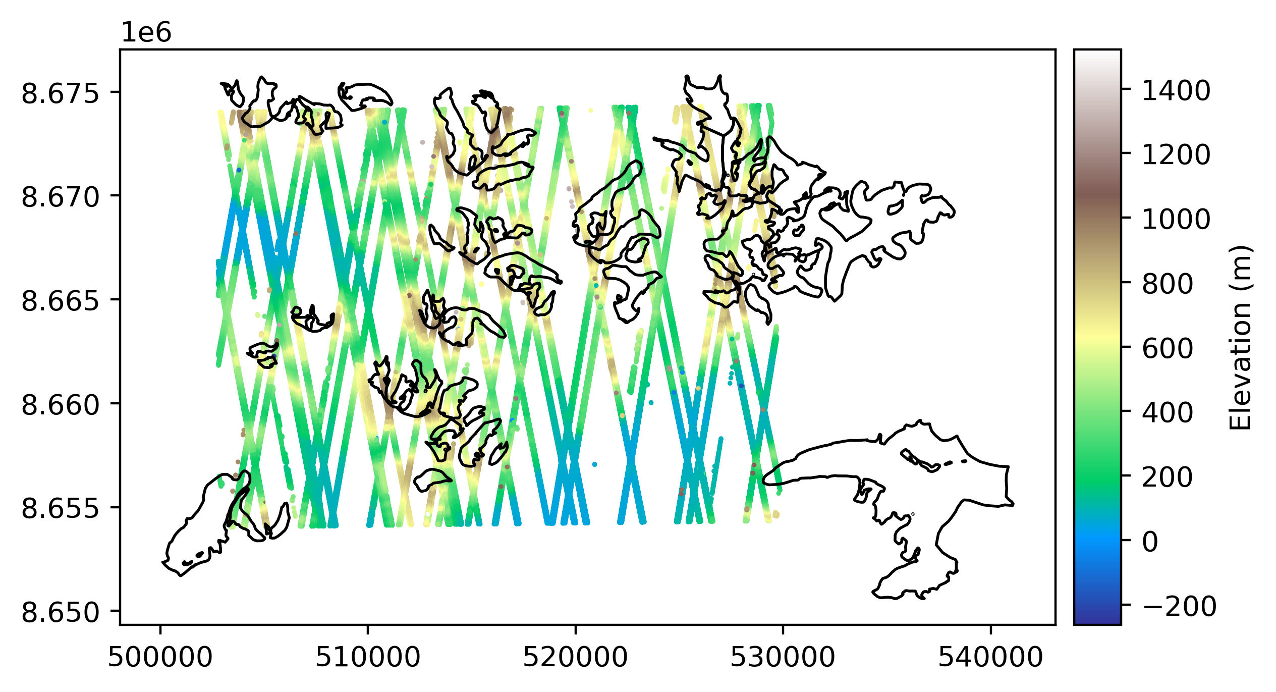
Plotting an elevation point cloud is done using plot(), and can be done alongside a raster or vector file.
# Open a vector file of glacier outlines near the EPC
import geoutils as gu
fn_glacier_outlines = xdem.examples.get_path("longyearbyen_glacier_outlines")
vect_gla = gu.Vector(fn_glacier_outlines)

# Reproject to local projected CRS
epc = epc.reproject(crs=epc.get_metric_crs())

# Crop outlines to those intersecting the EPC
vect_gla = vect_gla.crop(epc)

# Plot the DEM and the vector file
epc.plot(cmap="terrain", markersize=0.5, cbar_title="Elevation (m)")
vect_gla.plot(epc, ec="k", fc="none")  # We pass the EPC as reference for the plot CRS
Vertical referencing#
The vertical reference of an EPC is stored in vcrs, and derived either from its
crs (if 3D) or assessed from the DEM product name or user-input during instantiation.
# Check vertical CRS of dataset
epc.vcrs
'Ellipsoid'
In this case, the elevation point cloud is using a 3D CRS extended from the ellipsoid. To override manually with another vertical CRS,
set_vcrs is used. Then, to transform into another vertical CRS, use to_vcrs.
# Transform to the EGM96 geoid
epc = epc.to_vcrs("EGM96")
Note
For more details on vertical referencing, see the Vertical referencing page.
Statistics#
The get_stats() method allows to extract statistical information from a point cloud in a dictionary.
Get all statistics in a dict:
epc.get_stats()
{'Mean': np.float32(360.54987),
 'Median': np.float32(341.75214),
 'Max': np.float32(1489.6226),
 'Min': np.float32(-295.53012),
 'Sum': np.float32(6.3464708e+07),
 'Sum of squares': np.float32(3.3354668e+10),
 '90th percentile': np.float32(705.9401),
 'LE90': np.float32(754.7908),
 'IQR': np.float32(402.3305),
 'NMAD': np.float32(298.48083),
 'RMSE': np.float32(435.30618),
 'Standard deviation': np.float32(243.91655),
 'Valid count': np.int64(176022),
 'Total count': 176022,
 'Percentage valid points': np.float64(100.0)}
The point cloud statistics functionalities in xDEM are based on those in GeoUtils. For more information on computing statistics, please refer to GeoUtils’ documentation.
Coregistration#
3D coregistration is performed with coregister_3d(), which aligns the
EPC to a DEM (or vice versa) using a pipeline defined with a Coreg
object (defaults to horizontal and vertical shifts).
Important
Coregistration in xDEM currently support only EPC–DEM or DEM–DEM inputs, because coregistering two sparse EPCs is rarely useful and
dense EPCs (like lidar point clouds) reach similar coregistration accuracy when converted to a DEM (e.g. using grid()).
# A reference DEM to the elevation point cloud
filename_ref = xdem.examples.get_path("longyearbyen_ref_dem")
dem_ref = xdem.DEM(filename_ref)
epc = epc.reproject(dem_ref)
# Coregister (horizontal and vertical shifts)
epc_aligned = epc.coregister_3d(dem_ref, xdem.coreg.LZD())
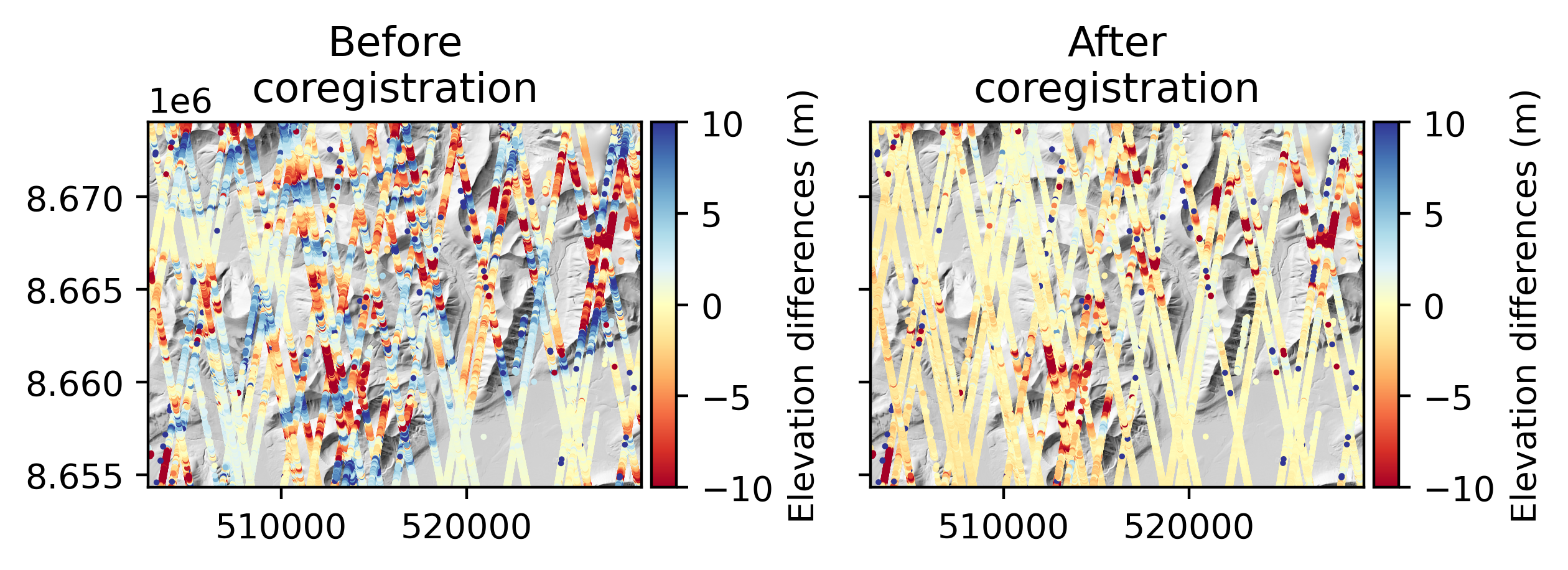
# Plot the elevation change before/after coregistration over a hillshade
hs = dem_ref.hillshade()
dh_before = epc - dem_ref.interp_points(epc)
dh_after = epc_aligned - dem_ref.interp_points(epc_aligned)
# Remove outliers
# dh_before[gu.stats.nmad(dh_before) < 3] = np.nan
# dh_after[gu.stats.nmad(dh_after) < 3] = np.nan
import matplotlib.pyplot as plt
f, ax = plt.subplots(1, 2)
ax[0].set_title("Before\ncoregistration")
hs.plot(ax=ax[0], cmap="Greys_r", add_cbar=False)
dh_before.plot(ax=ax[0], cmap='RdYlBu', vmin=-10, vmax=10, markersize=0.5, cbar_title="Elevation differences (m)")
ax[1].set_title("After\ncoregistration")
hs.plot(ax=ax[1], cmap="Greys_r", add_cbar=False)
dh_after.plot(ax=ax[1], cmap='RdYlBu', vmin=-10, vmax=10, markersize=0.5, cbar_title="Elevation differences (m)")
_ = ax[1].set_yticklabels([])
plt.tight_layout()
Note
For more details on building coregistration pipelines and accessing metadata, see the Coregistration page.