The digital elevation model (DEM)#
Below, a summary of the DEM object and its methods.
Object definition and attributes#
A DEM is a Raster with an additional georeferenced vertical dimension stored in the attribute vcrs.
It inherits the four main attributes of Raster which are data,
transform, crs and nodata.
Many other useful raster attributes and methods are available through the Raster object, such as
bounds, res, reproject() and crop() .
Tip
The complete list of Raster attributes and methods can be found in GeoUtils’ API and more info on rasters on GeoUtils’ Raster documentation page.
Open and save#
A DEM is opened by instantiating with either a str, a pathlib.Path, a rasterio.io.DatasetReader or a
rasterio.io.MemoryFile, as for a Raster.
import xdem

# Instantiate a DEM from a filename on disk
filename_dem = xdem.examples.get_path("longyearbyen_ref_dem")
dem = xdem.DEM(filename_dem)
dem
DEM(
  data=not_loaded; shape on disk (1, 985, 1332); will load (985, 1332)
  transform=| 20.00, 0.00, 502810.00|
            | 0.00,-20.00, 8674030.00|
            | 0.00, 0.00, 1.00|
  crs=EPSG:25833
  nodata=-9999.0)
Detailed information on the DEM is printed using info(), along with basic statistics using stats=True:
# Print details of raster
dem.info(stats=True)
Driver:               GTiff
Opened from file:     /home/docs/checkouts/readthedocs.org/user_builds/xdem-ould-a/checkouts/latest/xdem/example_data/Longyearbyen/data/DEM_2009_ref.tif
Filename:             /home/docs/checkouts/readthedocs.org/user_builds/xdem-ould-a/checkouts/latest/xdem/example_data/Longyearbyen/data/DEM_2009_ref.tif
Loaded?               False
Modified since load?  False
Grid size:            1332, 985
Number of bands:      1
Data types:           float32
Coordinate system:    ['EPSG:25833', 'None']
Nodata value:         -9999.0
Pixel interpretation: Area
Pixel size:           20.0, 20.0
Upper left corner:    502810.0, 8674030.0
Lower right corner:   529450.0, 8654330.0

Statistics:
Mean                   : 378.05
Median                 : 360.65
Max                    : 1022.21
Min                    : 8.05
Sum                    : 496010560.00
Sum of squares         : 265449996288.00
90th percentile        : 724.54
LE90                   : 766.59
IQR                    : 391.71
NMAD                   : 290.22
RMSE                   : 449.80
Standard deviation     : 243.72
Valid count            : 1312020.00
Total count            : 1312020.00
Percentage valid points: 100.00
Important
The DEM data array remains implicitly unloaded until data is called. For instance, here, calling info() with stats=True automatically loads the array in-memory.
The georeferencing metadata (transform, crs, nodata), however, is always loaded. This allows to pass it effortlessly to other objects requiring it for geospatial operations (reproject-match, rasterizing a vector, etc).
A DEM is saved to file by calling to_file() with a str or a pathlib.Path.
# Save raster to disk
dem.to_file("mydem.tif")
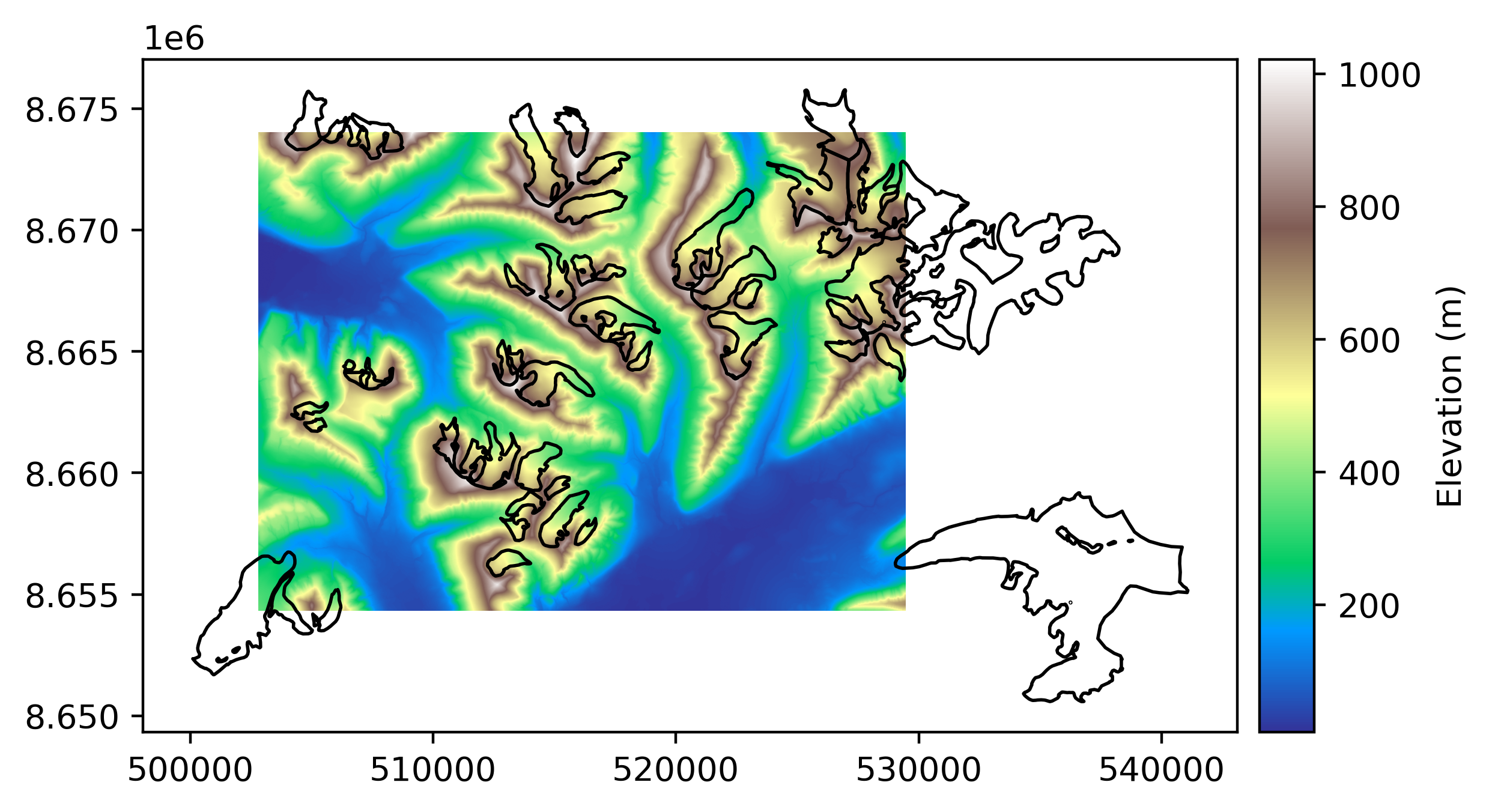
Plotting#
Plotting a DEM is done using plot(), and can be done alongside a vector file.
# Open a vector file of glacier outlines near the DEM
import geoutils as gu
fn_glacier_outlines = xdem.examples.get_path("longyearbyen_glacier_outlines")
vect_gla = gu.Vector(fn_glacier_outlines)

# Crop outlines to those intersecting the DEM
vect_gla = vect_gla.crop(dem)

# Plot the DEM and the vector file
dem.plot(cmap="terrain", cbar_title="Elevation (m)")
vect_gla.plot(dem, ec="k", fc="none")  # We pass the DEM as reference for the plot CRS
Vertical referencing#
The vertical reference of a DEM is stored in vcrs, and derived either from its
crs (if 3D) or assessed from the DEM product name during instantiation.
# Check vertical CRS of dataset
dem.vcrs
In this case, the DEM has no defined vertical CRS, which is quite common. To set the vertical CRS manually,
use set_vcrs. Then, to transform into another vertical CRS, use to_vcrs.
# Define the vertical CRS as the 3D ellipsoid of the 2D CRS
dem.set_vcrs("Ellipsoid")
# Transform to the EGM96 geoid
dem.to_vcrs("EGM96")
DEM(
  data=[[552.844970703125 561.4555053710938 566.9647827148438 ...
         244.73574829101562 255.0602569580078 264.2195739746094]
        [553.3552856445312 562.0689086914062 571.1232299804688 ...
         244.90061950683594 256.1825866699219 266.5284729003906]
        [552.4747314453125 561.7349853515625 570.4039916992188 ...
         243.29054260253906 253.91836547851562 264.7453918457031]
        ...
        [327.612548828125 326.80401611328125 325.9011535644531 ...
         526.854736328125 529.5508422851562 533.6632080078125]
        [328.2633361816406 327.5744934082031 326.6269836425781 ...
         512.1184692382812 514.7266845703125 518.1988525390625]
        [329.04254150390625 328.2438659667969 327.3596496582031 ...
         497.5435485839844 500.67388916015625 505.9179992675781]]
  transform=| 20.00, 0.00, 502810.00|
            | 0.00,-20.00, 8674030.00|
            | 0.00, 0.00, 1.00|
  crs=EPSG:25833
  nodata=-9999.0)
Note
For more details on vertical referencing, see the Vertical referencing page.
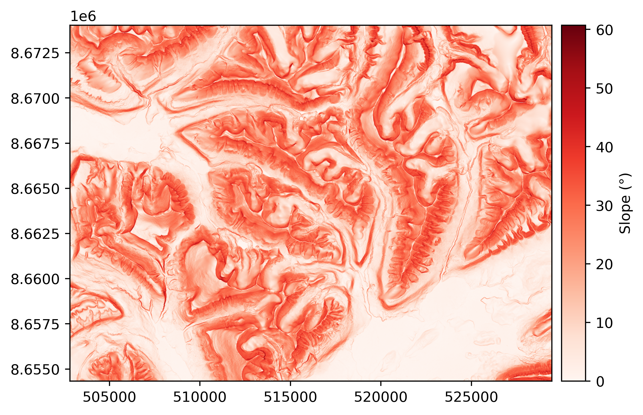
Terrain attributes#
A wide range of terrain attributes can be derived from a DEM, with several methods and options available,
by calling the function corresponding to the attribute name such as slope().
# Derive slope using the Zevenberg and Thorne (1987) method
slope = dem.slope(surface_fit="ZevenbergThorne")
slope.plot(cmap="Reds", cbar_title="Slope (°)")
Note
For the full list of terrain attributes, see the Terrain attributes page.
Statistics#
The get_stats() method allows to extract statistical information from a DEM in a dictionary.
Get all statistics in a dict:
dem.get_stats()
{'Mean': np.float64(378.0510662947211),
 'Median': np.float32(360.64624),
 'Max': np.float32(1022.211),
 'Min': np.float32(8.052481),
 'Sum': np.float32(4.9601056e+08),
 'Sum of squares': np.float32(2.6545e+11),
 '90th percentile': np.float64(724.5404052734376),
 'LE90': np.float64(766.594490814209),
 'IQR': np.float32(391.70935),
 'NMAD': np.float32(290.22385),
 'RMSE': np.float64(449.8017431289339),
 'Standard deviation': np.float64(243.71907060653254),
 'Valid count': np.int64(1312020),
 'Total count': 1312020,
 'Percentage valid points': np.float64(100.0)}
The DEM statistics functionalities in xDEM are based on those in GeoUtils. For more information on computing statistics, please refer to GeoUtils’ documentation.
Coregistration#
3D coregistration is performed with coregister_3d(), which aligns the
DEM to another DEM or EPC using a pipeline defined with a Coreg
object (defaults to horizontal and vertical shifts).
# Another DEM to-be-aligned to the first one
filename_tba = xdem.examples.get_path("longyearbyen_tba_dem")
dem_tba = xdem.DEM(filename_tba)

# Coregister (horizontal and vertical shifts)
dem_tba_coreg = dem_tba.coregister_3d(dem, xdem.coreg.NuthKaab() + xdem.coreg.VerticalShift())

# Plot the elevation change of the DEM due to coregistration
dh_tba = dem_tba - dem_tba_coreg.reproject(dem_tba, silent=True)
dh_tba.plot(cmap="Spectral", cbar_title="Elevation change due to coreg (m)")

Note
For more details on building coregistration pipelines and accessing metadata, see the Coregistration page.
Uncertainty analysis#
Estimation of DEM-related uncertainty can be performed with estimate_uncertainty(), which estimates both
an error map considering variable per-pixel errors and the spatial correlation of errors. The workflow relies
on an independent elevation data object that is assumed to have either much finer or similar precision, and uses
stable terrain as a proxy.
# Estimate elevation uncertainty assuming both DEMs have similar precision
sig_dem, rho_sig = dem.estimate_uncertainty(dem_tba_coreg, precision_of_other="same", random_state=42)

# The error map variability is estimated from slope and curvature by default
sig_dem.plot(cmap="Purples", cbar_title=r"Random error in elevation (1$\sigma$, m)")

# The spatial correlation function represents how much errors are correlated at a certain distance
print("Elevation errors at a distance of 1 km are correlated at {:.2f} %.".format(rho_sig(1000) * 100))
Elevation errors at a distance of 1 km are correlated at 11.28 %.

Note
We use random_state to ensure a fixed randomized output. It is only necessary if you need your results to be exactly reproductible.
For more details on quantifying random and structured errors, see the Uncertainty analysis page.